Prerequisites
This course assumes that you already know Python. The scipy-lectures give an introduction to Python.
Tip
This page gives an introduction to statistics with Python. It is useful to get acquainted with data representations in Python. In terms of experimental psychology, the patterns demonstrated here can be applied to simple dataset that arise from psychophysics, or reaction time experiments. We will see how to process efficiently more complex data as produced by brain imaging in the next course.
Tip
We will be working in the interactive Python prompt, IPython. You can either start it by itself, or in the spyder environment.
In this document, the Python prompts are represented with the sign “>>>”. If you need to copy-paste code, you can click on the top right of the code blocks, to hide the prompts and the outputs.
We have the reaction times in a psychophysical experiment:
474.688 506.445 524.081 530.672 530.869 566.984 582.311 582.940 603.574 792.358
In Python, we will represent them using a numerical “array”, with the numpy module:
>>> import numpy as np
>>> x = np.array([474.688, 506.445, 524.081, 530.672, 530.869, 566.984, 582.311, 582.940, 603.574, 792.358])
We can access the elements of x with indexing, starting at 0:
>>> x[0]    # First element
474.68799999999999
>>> x[:3]   # Up to the third element
array([ 474.688,  506.445,  524.081])
>>> x[-1]   # Last element
792.35799999999995
Mathematical operations on arrays are done using the numpy module:
>>> np.max(x)
792.35799999999995
>>> np.sum(x[:3])
1505.2139999999999
>>> np.mean(x)
569.49219999999991
>>> np.log(x)
array([ 6.16265775,  6.22741573,  6.26164625,  6.27414413,  6.27451529,
        6.34033108,  6.36700467,  6.36808427,  6.40286865,  6.67501331])
Finding help
Exercise
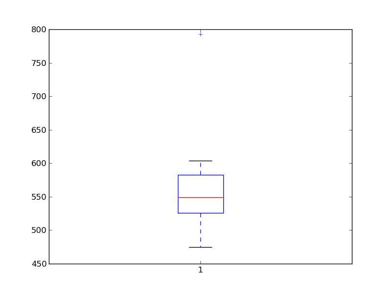
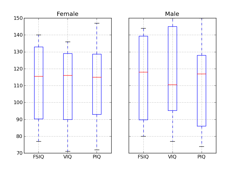
Basic plotting is done with matplotlib:
>>> from matplotlib import pyplot as plt
>>> plt.boxplot(x)
Hint
If a window doesn’t display, you need to call plt.show().
Under IPython, type %matplotlib to have plots display automatically.


See also
Matplotlib is very rich and can be controlled in detail. See the scipy lectures for more details.
We have a CSV file giving observations of brain size and weight and IQ (Willerman et al. 1991):
"";"Gender";"FSIQ";"VIQ";"PIQ";"Weight";"Height";"MRI_Count"
"1";"Female";133;132;124;"118";"64.5";816932
"2";"Male";140;150;124;".";"72.5";1001121
"3";"Male";139;123;150;"143";"73.3";1038437
"4";"Male";133;129;128;"172";"68.8";965353
The data are a mixture of numerical and categorical values. We will use pandas to manipulate them:
>>> import pandas
>>> data = pandas.read_csv('examples/brain_size.csv', sep=';', na_values=".")
>>> print data
    Unnamed: 0  Gender  FSIQ  VIQ  PIQ  Weight  Height  MRI_Count
0            1  Female   133  132  124     118    64.5     816932
1            2    Male   140  150  124     NaN    72.5    1001121
2            3    Male   139  123  150     143    73.3    1038437
3            4    Male   133  129  128     172    68.8     965353
4            5  Female   137  132  134     147    65.0     951545
...
Warning
Missing values
The weight of the second individual is missing in the CSV file. If we don’t specify the missing value (NA = not available) marker, we will not be able to do statistics on the weight.
data is a pandas dataframe, that resembles R’s dataframe:
>>> print data['Gender']
0     Female
1       Male
2       Male
3       Male
4     Female
...
>>> gender_data = data.groupby('Gender')
>>> print gender_data.mean()
        Unnamed: 0   FSIQ     VIQ     PIQ      Weight     Height  MRI_Count
Gender
Female       19.65  111.9  109.45  110.45  137.200000  65.765000   862654.6
Male         21.35  115.0  115.25  111.60  166.444444  71.431579   954855.4


>>> # More manual, but more versatile
>>> for name, value in gender_data['VIQ']:
...     print name, np.mean(value)
Female 109.45
Male 115.25

>>> # Simpler selector
>>> data[data['Gender'] == 'Female']['VIQ'].mean()
109.45
Exercise
What is the mean value for VIQ for the full population?
How many males/females were included in this study?
Hint use ‘tab completion’ to find out the methods that can be called, instead of ‘mean’ in the above example.
What is the average value of MRI counts expressed in log units, for males and females?
Pandas comes with some plotting tools (that use matplotlib behind the scene) to display statistics on dataframes:
>>> from pandas.tools import plotting
>>> plotting.scatter_matrix(data[['Weight', 'Height', 'MRI_Count']])
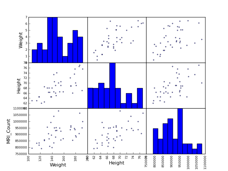
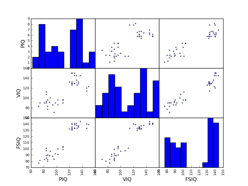
>>> plotting.scatter_matrix(data[['PIQ', 'VIQ', 'FSIQ']])
Exercise
Plot the scatter matrix for males only, and for females only. Do you think that the 2 sub-populations correspond to gender?
For simple statistical tests, we will use the stats sub-module of scipy:
>>> from scipy import stats
See also
Scipy is a vast library. For a tutorial covering the whole scope of scipy, see http://scipy-lectures.github.io/
scipy.stats.ttest_1samp() tests if observations are drawn from a Gaussian distributions of given population mean. It returns the T statistic, and the p-value (see the function’s help):
>>> stats.ttest_1samp(data['VIQ'], 0)
(30.088099970849338, 1.3289196468727784e-28)
Tip
With a p-value of 10^-28 we can claim that the population mean for the IQ (VIQ measure) is not 0.
Exercise
Is the test performed above one-sided or two-sided? Which one should we use, and what is the corresponding p-value?
We have seen above that the mean VIQ in the male and female populations were different. To test if this is significant, we do a 2-sample t-test with scipy.stats.ttest_ind():
>>> female_viq = data[data['Gender'] == 'Female']['VIQ']
>>> male_viq = data[data['Gender'] == 'Male']['VIQ']
>>> stats.ttest_ind(female_viq, male_viq)
(-0.77261617232750124, 0.44452876778583217)
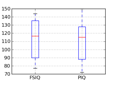
PIQ, VIQ, and FSIQ give 3 measures of IQ. Let us test if FISQ and PIQ are significantly different. We need to use a 2 sample test:
>>> stats.ttest_ind(data['FSIQ'], data['PIQ'])
(0.46563759638096403, 0.64277250094148408)
The problem with this approach is that is forgets that there are links between observations: FSIQ and PIQ are measure on the same individuals. Thus the variance due to inter-subject variability is confounding, and can be removed, using a “paired test”, or “repeated measure test”:
>>> stats.ttest_rel(data['FSIQ'], data['PIQ'])
(1.7842019405859857, 0.082172638183642358)
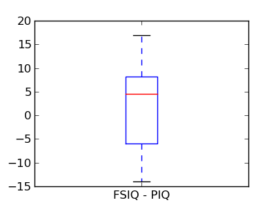
This is equivalent to a 1-sample test on the difference:
>>> stats.ttest_1samp(data['FSIQ'] - data['PIQ'], 0)
(1.7842019405859857, 0.082172638183642358)
T-tests assume Gaussian errors. We can use a Wilcoxon signed-rank test, that relaxes this assumption:
>>> stats.wilcoxon(data['FSIQ'], data['PIQ'])
(274.5, 0.034714577290489719)
Note
The corresponding test in the non paired case is the Mann–Whitney U test, scipy.stats.mannwhitneyu().
Exercice
Given two set of observations, x and y, we want to test the hypothesis that y is a linear function of x. In other terms:
where e is observation noise. We will use the statmodels module to:
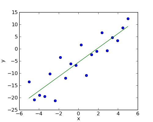
First, we generate simulated data according to the model:
>>> x = np.linspace(-5, 5, 20)
>>> np.random.seed(1)
>>> # normal distributed noise
>>> y = -5 + 3*x + 4 * np.random.normal(size=x.shape)
>>> # Create a data frame containing all the relevant variables
>>> data = pandas.DataFrame({'x': x, 'y': y})
Specify an OLS model and fit it:
>>> # The following will work only with a recent version of statsmodels
>>> from statsmodels.formula.api import ols
>>> model = ols("y ~ x", data).fit()
>>> print(model.summary())
                            OLS Regression Results
==============================================================================
Dep. Variable:                      y   R-squared:                       0.804
Model:                            OLS   Adj. R-squared:                  0.794
Method:                 Least Squares   F-statistic:                     74.03
Date:                ...                Prob (F-statistic):           8.56e-08
Time:                        ...        Log-Likelihood:                -57.988
No. Observations:                  20   AIC:                             120.0
Df Residuals:                      18   BIC:                             122.0
Df Model:                           1
==============================================================================
                 coef    std err          t      P>|t|      [95.0% Conf. Int.]
------------------------------------------------------------------------------
Intercept     -5.5335      1.036     -5.342      0.000        -7.710    -3.357
x              2.9369      0.341      8.604      0.000         2.220     3.654
==============================================================================
Omnibus:                        0.100   Durbin-Watson:                   2.956
Prob(Omnibus):                  0.951   Jarque-Bera (JB):                0.322
Skew:                          -0.058   Prob(JB):                        0.851
Kurtosis:                       2.390   Cond. No.                         3.03
==============================================================================
Exercise
Retrieve the estimated parameters from the model above. Hint: use tab-completion to find the relevent attribute.
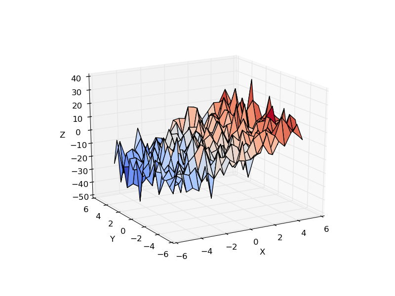
Consider a linear model explaining a variable z (the dependent variable) with 2 variables x and y:
Such a model can be seen in 3D as fitting a plane to a cloud of (x, y, z) points.
Example: the iris data
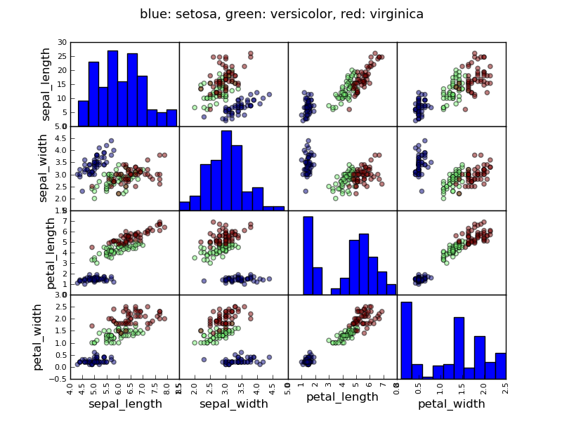
>>> data = pandas.read_csv('examples/iris.csv')
>>> model = ols('sepal_width ~ name + petal_length', data).fit()
>>> print(model.summary())
                            OLS Regression Results
==============================================================================
Dep. Variable:            sepal_width   R-squared:                       0.478
Model:                            OLS   Adj. R-squared:                  0.468
Method:                 Least Squares   F-statistic:                     44.63
Date:                ...                Prob (F-statistic):           1.58e-20
Time:                        ...        Log-Likelihood:                -38.185
No. Observations:                 150   AIC:                             84.37
Df Residuals:                     146   BIC:                             96.41
Df Model:                           3
===============================================================================...
                         coef    std err          t     P>|t|  [95.0% Conf. Int.]
-------------------------------------------------------------------------------...
Intercept              2.9813      0.099     29.989     0.000      2.785     3.178
name[T.versicolor]    -1.4821      0.181     -8.190     0.000     -1.840    -1.124
name[T.virginica]     -1.6635      0.256     -6.502     0.000     -2.169    -1.158
petal_length           0.2983      0.061      4.920     0.000      0.178     0.418
==============================================================================
Omnibus:                        2.868   Durbin-Watson:                   1.753
Prob(Omnibus):                  0.238   Jarque-Bera (JB):                2.885
Skew:                          -0.082   Prob(JB):                        0.236
Kurtosis:                       3.659   Cond. No.                         54.0
==============================================================================
In the above iris example, we wish to test if the petal length is different between versicolor and virginica, after removing the effect of sepal width. This can be formulated as testing the difference between the coefficient associated to versicolor and virginica in the linear model estimated above (it is an Analysis of Variance, ANOVA). For this, we write a vector of ‘contrast’ on the parameters estimated: we want to test “name[T.versicolor] - name[T.virginica]”, with an ‘F-test’:
>>> print(model.f_test([0, 1, -1, 0]))
<F test: F=array([[ 3.24533535]]), p=[[ 0.07369059]], df_denom=146, df_num=1>
Is this difference significant?
Exercice
Going back to the brain size + IQ data, test if the VIQ of male and female are different after removing the effect of brain size, height and weight.


