The aim of this exercise is to represent the time series of conditions that the experimenter imposes on the subject. It is important to get a good picture of the shape of this time series, because this is the shape of the modulation of the measured signal that we expect to see in brain regions involved in the targetted process.
Basically you need to know in which condition the subject was when each measurement was recorded.
The best way to make sense of the description of the experimental paradigm is actually to get a pencil and a piece of paper and to start scribbling, but here, we are going to do it with python.
Relevant information in the example:

Python source code: plot_time_series.py
import numpy as np
import matplotlib.pyplot as plt
from matplotlib.patches import Polygon
from matplotlib.collections import PatchCollection
# Considering we repeat 8 times a basic pattern "42s OFF, then 42s ON"
stim=np.hstack([np.zeros(42),np.ones(42)])
stim=np.tile(stim,8)
# check the total time
stim.shape
# prepare a nice figure
fig=plt.figure()
ax=fig.add_axes([.1,.1,.8,.8])
ax.set_title('Rest and audio stim alternating for 16 blocks')
ax.set_yticks([0,1])
ax.set_yticklabels(['OFF','ON'])
ax.set_ylabel('Condition: audio stimulation')
ax.set_xlabel('Time (second)')
plt.axis([-1,stim.shape[0]+1,-0.1,1.25])
# then plot
plt.plot(stim);
# Now let's represent the time series of measurements.
#
# definition: the repetition time (RT) is the time it takes for the scanner
# to do two consecutive measurements in the same voxel, in our case RT = 7s.
#
# The experimental manipulation starts at the 4th scan, which means the
# image acquisition started 3*7 seconds before.
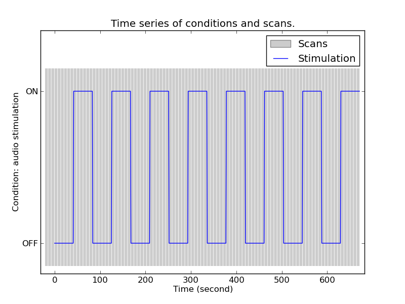
fig=plt.figure()
ax=fig.add_axes([.1,.1,.8,.8],title='Time series of conditions and scans.',)
plt.plot(stim)
plt.axis([-3*7-10,stim.shape[0]+10,-0.2,1.4])
ax.set_yticks([0,1])
ax.set_yticklabels(['OFF','ON'])
ax.set_ylabel('Condition: audio stimulation')
ax.set_xlabel('Time (second)')
#
# Here it's a bit tricky: we create a bunch of polygons and collect them
patches=[]
for ttl in np.arange(-3*7,42*16,7):
poly=Polygon(np.array([[ttl,-.15],[ttl,1.15],[ttl+6.05,1.15],[ttl+6.05,-.15]]),True)
patches.append(poly)
p=PatchCollection(patches,facecolor='0.5',edgecolor='none',alpha=0.4)
ax.add_collection(p)
# now the legend for which it's acutally easier to create dummy objects
# because the PatchCollection is not well supported by plt.legend
pp=plt.Rectangle((0,0),1,1,fc='0.5',ec='none',alpha=0.4)
l=plt.Line2D(np.array([0,1]),np.array([0,0]))
plt.legend([pp,l],["Scans","Stimulation"])
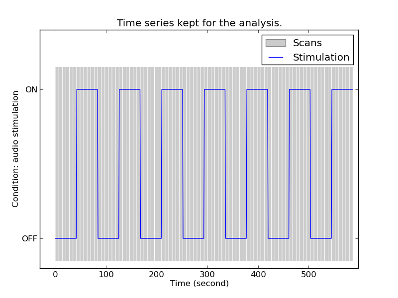
# Now 12 contaminated scans are discarded (on top of the 3 initial scans),
# thus 12*7 seconds have to be renoved from our time series of conditions
# in order to keep both time series with the same time reference:
# the beginning of the second stimulation basic pattern.
# Thus only 14 blocks are kept for the analysis.
stim=stim[12*7:]
stim.shape
fig=plt.figure()
ax=fig.add_axes([.1,.1,.8,.8],title='Time series kept for the analysis.',)
plt.plot(stim)
plt.axis([-3*7-10,stim.shape[0]+10,-0.2,1.4])
ax.set_yticks([0,1])
ax.set_yticklabels(['OFF','ON'])
ax.set_ylabel('Condition: audio stimulation')
ax.set_xlabel('Time (second)')
patches=[]
for ttl in np.arange(0,42*14,7):
poly=Polygon(np.array([[ttl,-.15],[ttl,1.15],[ttl+6.05,1.15],[ttl+6.05,-.15]]),True)
patches.append(poly)
p=PatchCollection(patches,facecolor='0.5',edgecolor='none',alpha=0.4)
ax.add_collection(p)
pp=plt.Rectangle((0,0),1,1,fc='0.5',ec='none',alpha=0.4)
l=plt.Line2D(np.array([0,1]),np.array([0,0]))
plt.legend([pp,l],["Scans","Stimulation"])
Total running time of the example: 1.09 seconds ( 0 minutes 1.09 seconds)
