Going back to the brain size + IQ data, test if the VIQ of male and female are different after removing the effect of brain size, height and weight.
Script output:
  OLS Regression Results
==============================================================================
Dep. Variable:                    VIQ   R-squared:                       0.246
Model:                            OLS   Adj. R-squared:                  0.181
Method:                 Least Squares   F-statistic:                     3.809
Date:                Mon, 02 Dec 2013   Prob (F-statistic):             0.0184
Time:                        22:10:29   Log-Likelihood:                -172.34
No. Observations:                  39   AIC:                             352.7
Df Residuals:                      35   BIC:                             359.3
Df Model:                           3
==================================================================================
                     coef    std err          t      P>|t|      [95.0% Conf. Int.]
----------------------------------------------------------------------------------
Intercept        166.6258     88.824      1.876      0.069       -13.696   346.948
Gender[T.Male]     8.8524     10.710      0.827      0.414       -12.890    30.595
MRI_Count          0.0002   6.46e-05      2.615      0.013      3.78e-05     0.000
Height            -3.0837      1.276     -2.417      0.021        -5.674    -0.494
==============================================================================
Omnibus:                        7.373   Durbin-Watson:                   2.109
Prob(Omnibus):                  0.025   Jarque-Bera (JB):                2.252
Skew:                           0.005   Prob(JB):                        0.324
Kurtosis:                       1.823   Cond. No.                     2.40e+07
==============================================================================

Warnings:
[1] The condition number is large, 2.4e+07. This might indicate that there are
strong multicollinearity or other numerical problems.
<F test: F=array([[ 0.68319608]]), p=[[ 0.41408784]], df_denom=35, df_num=1>
Python source code: plot_brain_size.py
import pandas
from statsmodels.formula.api import ols
data = pandas.read_csv('../brain_size.csv', sep=';', na_values='.')
model = ols('VIQ ~ Gender + MRI_Count + Height', data).fit()
print(model.summary())
# Here, we don't need to define a contrast, as we are testing a single
# coefficient of our model, and not a combination of coefficients.
# However, defining a contrast, which would then be a 'unit contrast',
# will give us the same results
print(model.f_test([0, 1, 0, 0]))
###############################################################################
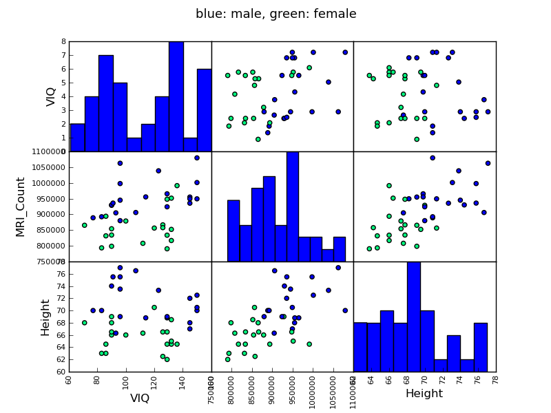
# Here we plot a scatter matrix to get intuitions on our results.
# This goes beyond what was asked in the exercise
# This plotting is useful to get an intuitions on the relationships between
# our different variables
from pandas.tools import plotting
import matplotlib.pyplot as plt
# Fill in the missing values for Height for plotting
data['Height'].fillna(method='pad', inplace=True)
# The parameter 'c' is passed to plt.scatter and will control the color
# The same holds for parameters 'marker', 'alpha' and 'cmap', that
# control respectively the type of marker used, their transparency and
# the colormap
plotting.scatter_matrix(data[['VIQ', 'MRI_Count', 'Height']],
c=(data['Gender'] == 'Female'), marker='o',
alpha=1, cmap='winter')
fig = plt.gcf()
fig.suptitle("blue: male, green: female", size=13)
plt.show()
Total running time of the example: 4.76 seconds ( 0 minutes 4.76 seconds)
