Ilustrate an analysis on a real dataset:
Script output:
  OLS Regression Results
==============================================================================
Dep. Variable:            sepal_width   R-squared:                       0.478
Model:                            OLS   Adj. R-squared:                  0.468
Method:                 Least Squares   F-statistic:                     44.63
Date:                Mon, 25 Nov 2013   Prob (F-statistic):           1.58e-20
Time:                        23:37:50   Log-Likelihood:                -38.185
No. Observations:                 150   AIC:                             84.37
Df Residuals:                     146   BIC:                             96.41
Df Model:                           3
======================================================================================
                         coef    std err          t      P>|t|      [95.0% Conf. Int.]
--------------------------------------------------------------------------------------
Intercept              2.9813      0.099     29.989      0.000         2.785     3.178
name[T.versicolor]    -1.4821      0.181     -8.190      0.000        -1.840    -1.124
name[T.virginica]     -1.6635      0.256     -6.502      0.000        -2.169    -1.158
petal_length           0.2983      0.061      4.920      0.000         0.178     0.418
==============================================================================
Omnibus:                        2.868   Durbin-Watson:                   1.753
Prob(Omnibus):                  0.238   Jarque-Bera (JB):                2.885
Skew:                          -0.082   Prob(JB):                        0.236
Kurtosis:                       3.659   Cond. No.                         54.0
==============================================================================
Testing the difference between effect of versicolor and virginica
<F test: F=array([[ 3.24533535]]), p=[[ 0.07369059]], df_denom=146, df_num=1>
Python source code: plot_iris_analysis.py
import matplotlib.pyplot as plt
import pandas
from pandas.tools import plotting
from statsmodels.formula.api import ols
# Load the data
data = pandas.read_csv('iris.csv')
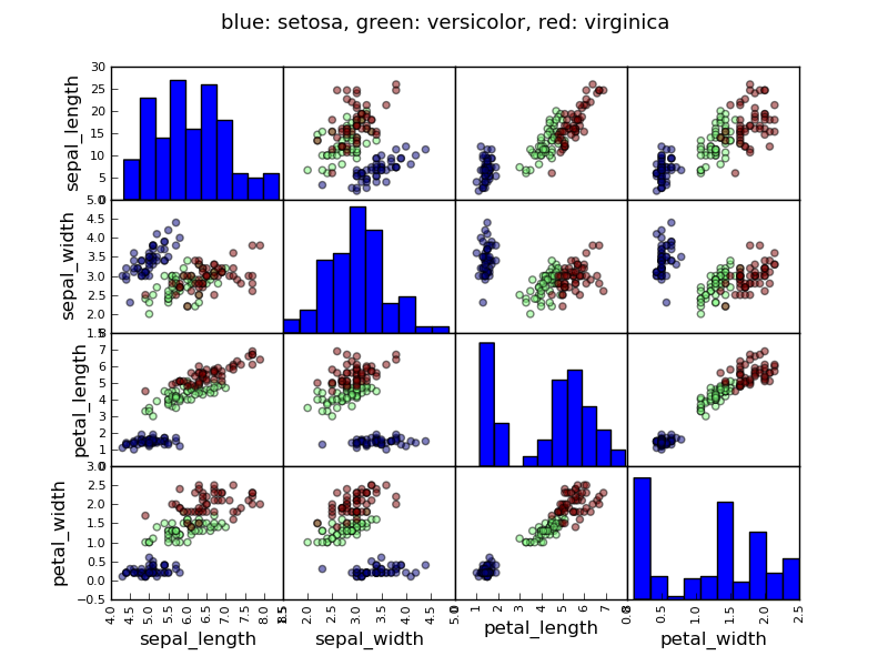
##############################################################################
# Plot a scatter matrix
# Express the names as categories
categories = pandas.Categorical(data['name'])
# The parameter 'c' is passed to plt.scatter and will control the color
plotting.scatter_matrix(data, c=categories.labels, marker='o')
fig = plt.gcf()
fig.suptitle("blue: setosa, green: versicolor, red: virginica", size=13)
##############################################################################
# Statistical analysis
# Let us try to explain the sepal length as a function of the petal
# width and the category of iris
model = ols('sepal_width ~ name + petal_length', data).fit()
print(model.summary())
# Now formulate a "contrast", to test if the offset for versicolor and
# virginica are identical
print('Testing the difference between effect of versicolor and virginica')
print(model.f_test([0, 1, -1, 0]))
plt.show()
Total running time of the example: 1.44 seconds ( 0 minutes 1.44 seconds)
